Sources

← back to the map

The sources used for this project are listed below. Keep in mind that the original sources are sometimes offered under different open licenses which should be consulted before making any use of them in a commercial project. Note that timetables and statistics were often digitized with large language models and most have only been spot checked so far. Carefully consult the original source before using them.

Projections

The map is drawn on a Pacific-centred frame running 66°E–206°E and 13°S–55°N — British India to Pearl Harbor, Sakhalin to northern Australia. Longitudes are normalised to 0–360 so the map is continuous across the antimeridian. Three projections are offered in Layers:

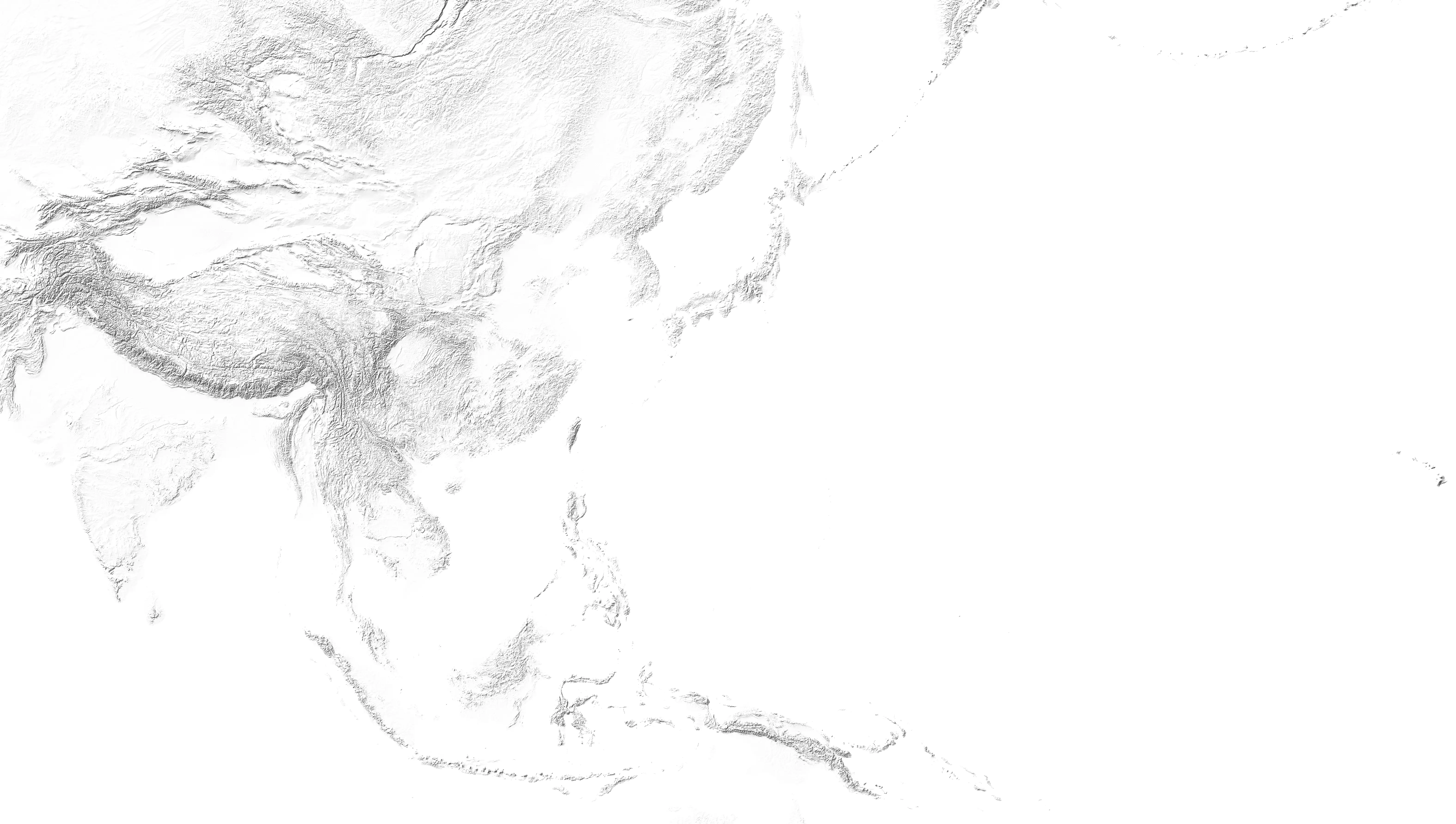
• Web Mercator, the sheet as built and the one the map opens on.
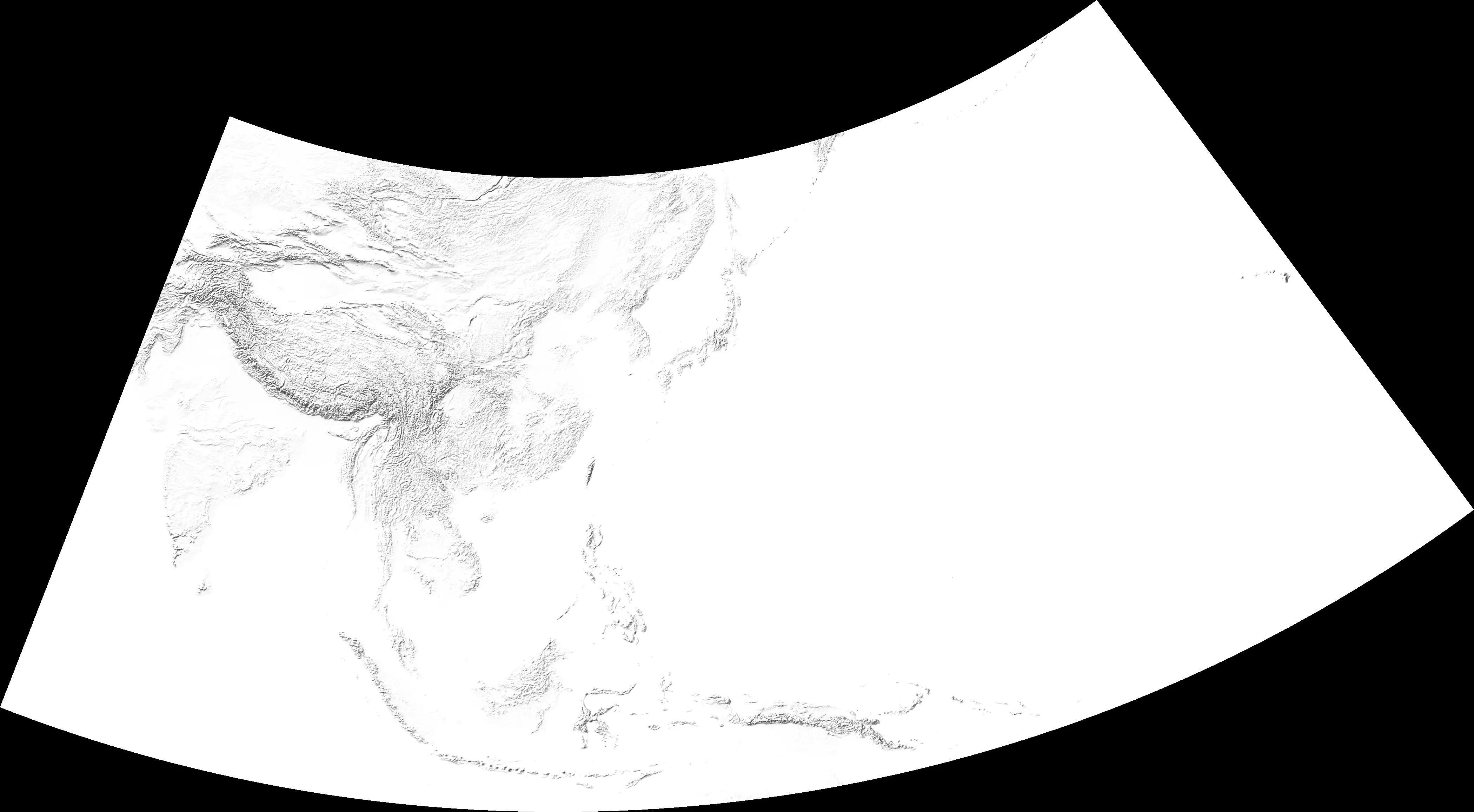
• Albers equal-area conic, on 117.5°E with standard parallels at 12.5°N and 37.5°N.
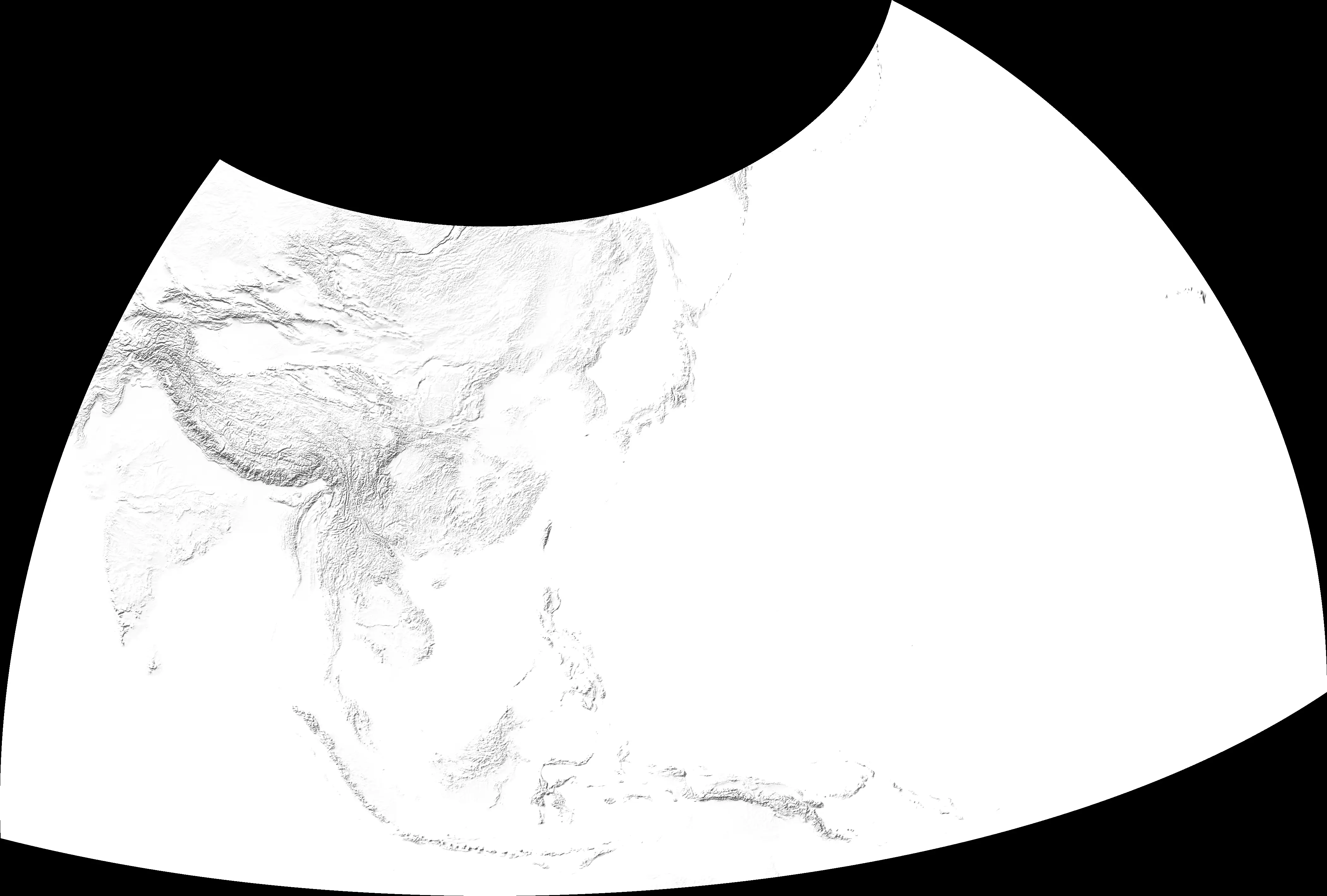
• Lambert azimuthal equal area, centred on 25°N 115°E.

Coastlines and Topography

• Most of the coastlines and national outlines are originally Natural Earth, except China's, which is derived from the Republican province sheet below, and Korea's coastline which came with the provincial boundaries below. The more detailed coastlines that load in some cases when you zoom in, as with various Pacific islands, are taken from OSM Coastlines.
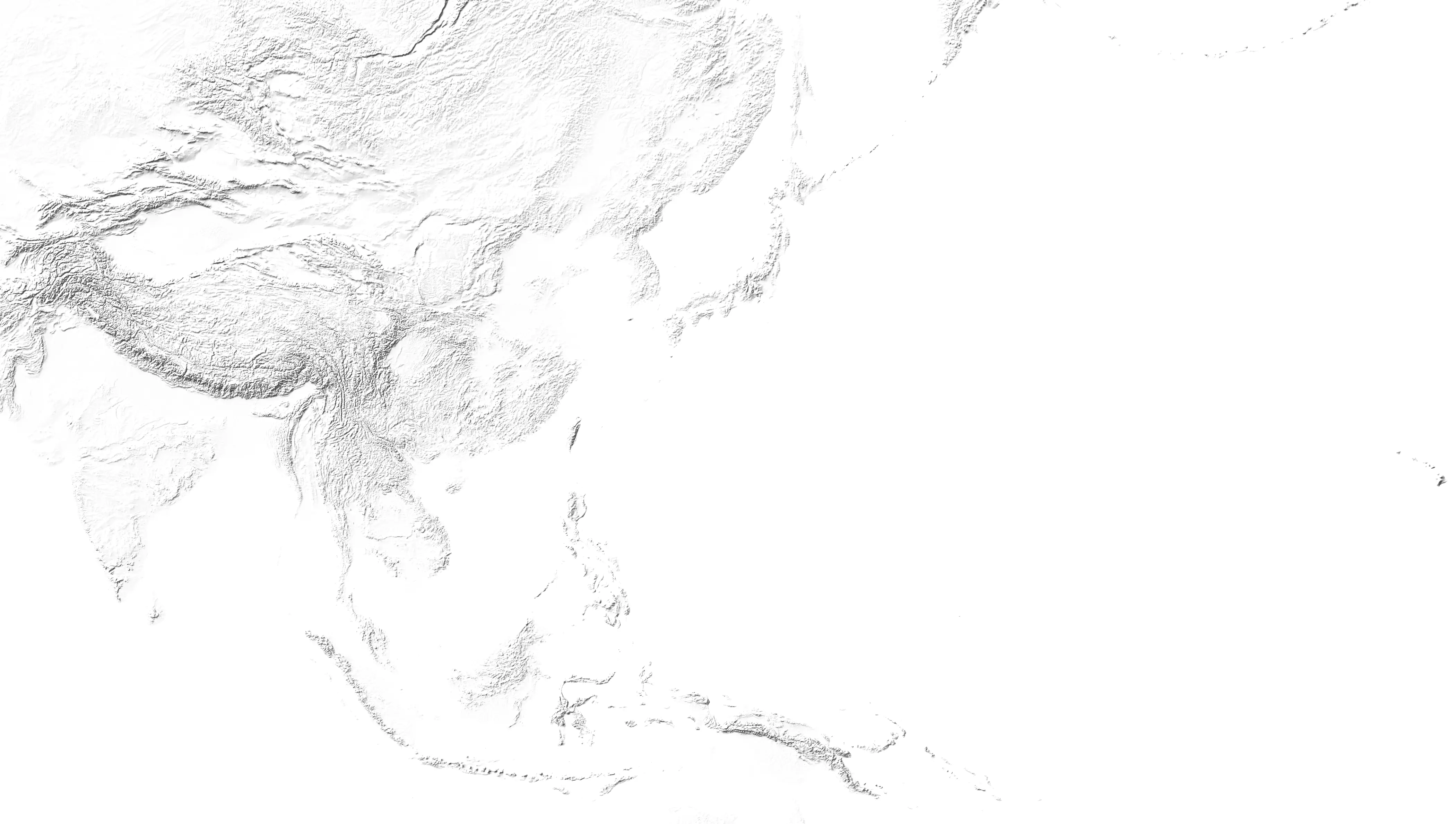
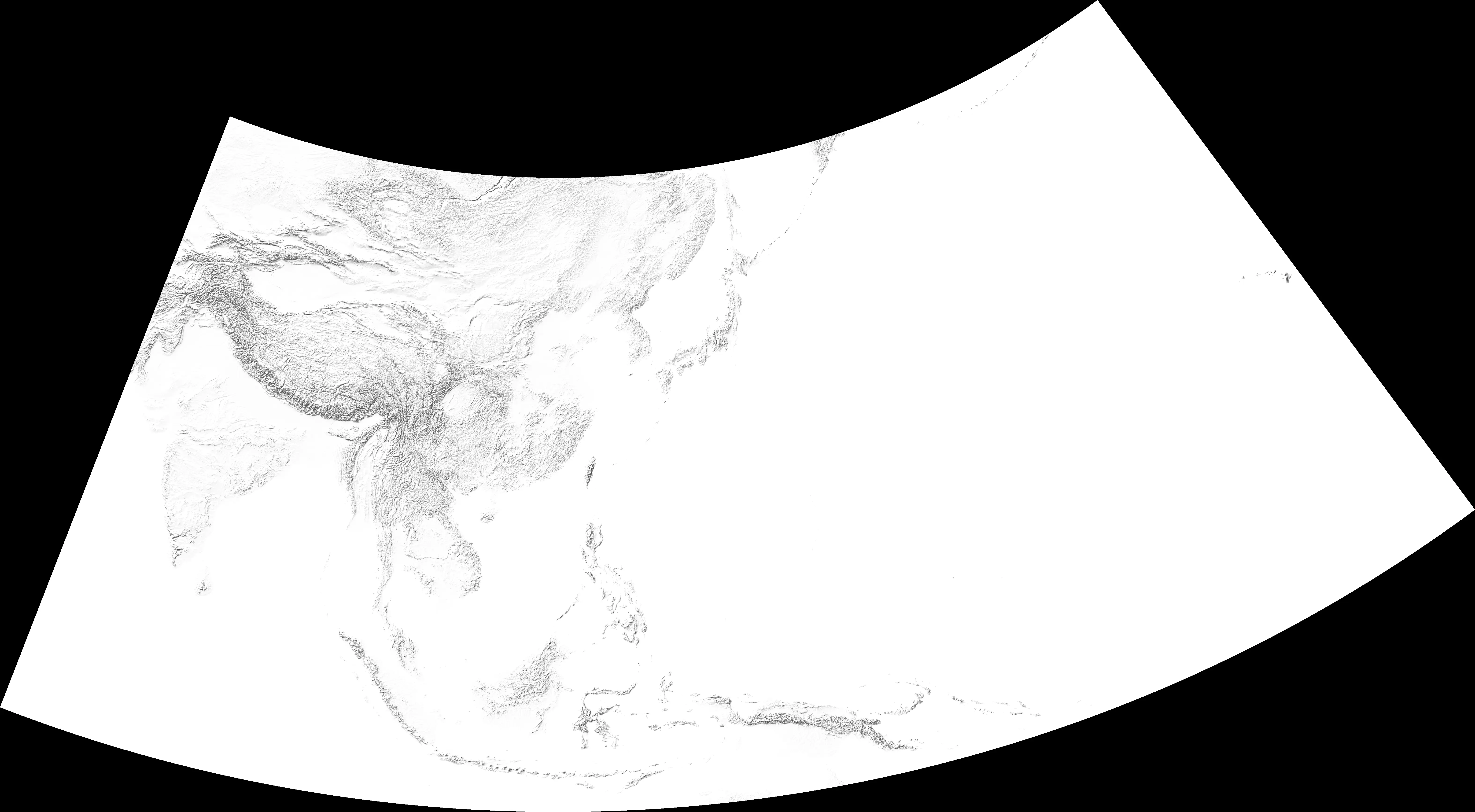
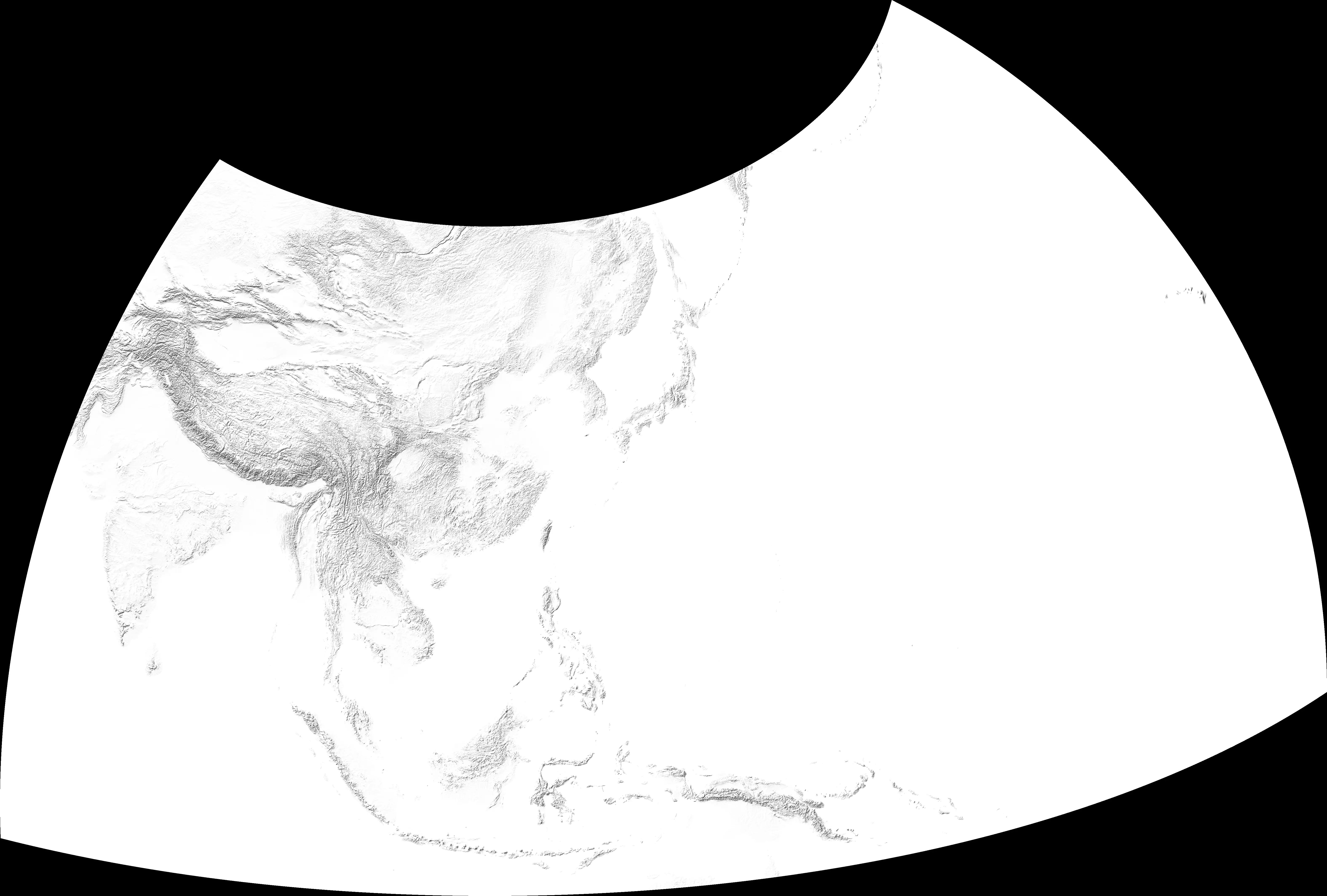
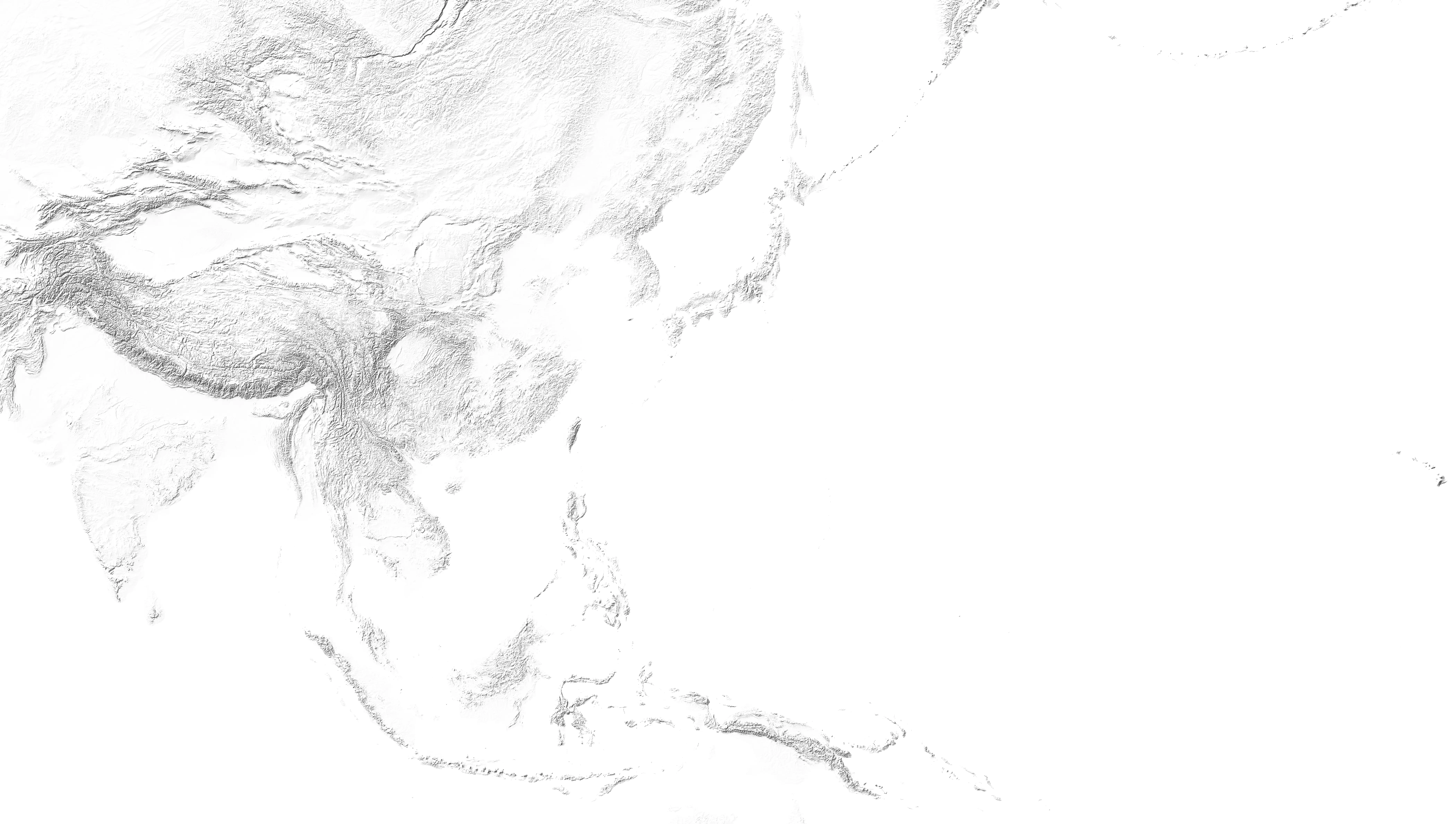
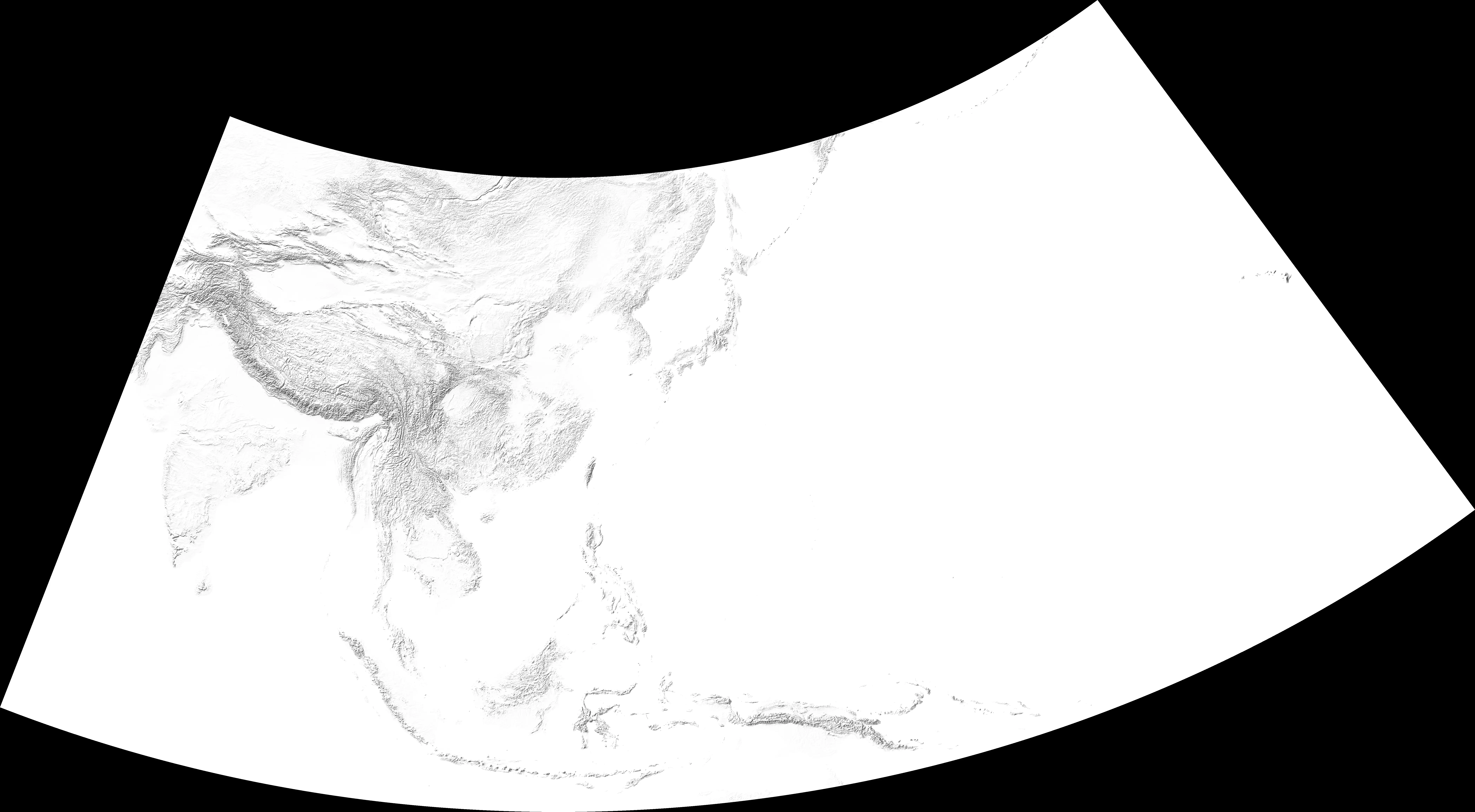
• Topography. Shaded relief after Natural Earth (public domain), SR_HR (1:10m, 1 arc-minute) — clipped to the map's frame and warped into each of the three projections the map offers. The sheet's flat water value is remapped to white.

Boundaries

• Natural Earth, 1:10m cultural vectors. A number of national outlines begin with Natural Earth and are modified from there. Public domain. github.com/nvkelso/natural-earth-vector
• Chinese Provincial Boundaries - This began with ENP-China — Chinese provincial boundaries, 1928–1945. Now this layer is only used for the coastline of China. Originally the provinces of China were used from this dataset but on further investigation, the version we had seems to show interior provinces (such as Shaanxi frontier along the Yellow River) significantly distant from where it should be. I decided to keep the coastlines from this layer for convenience and then redo the provinces from historical maps (see below). Christian Henriot (June 16, 2021). Administrative map of Republican China: Provinces (1912-1928). Elites, Networks and Power in modern China. Retrieved August 24, 2026 DOI A few more maps were consulted in drawing the provincial boundaries:
• 中華民國新地圖 交通及物產詳記 (1936 [earlier version 1928]) - HKUST Library .
• 中華民國新地圖 (1947) - Academia Sinica.
• 最新世界大地図 - David Rumsey Historical Map Collection, Fuchida, Tadayoshi, Saishin sekai daichizu: Shina zendo narabi fukin daichizu. Oshū gensei daichizu (1940) List No. 13462.003. David Rumsey
• French Indochina Boundaries - Traced from a 1945 OSS map. Traced from the map held at Stanford as bv890bn4231. The territory ceded to Thailand in May 1941 is drawn in the vector file as units of the federation on the 1930 sheet to make it easier to detach them for the 1942 map.
• Burma's administrative areas. The divisions and districts were drawn from the Imperial Gazetteer of India, Atlas: 1931, digitized by the University of Chicago Digital South Asia Library.
• The Netherlands Indies. Natural Earth coastlines with the administrative boundaries for the 1930 map and then modifications to fit the 1942 map drawn from Robert Cribb, Historical Atlas of Indonesia (2000), pp. 125-6 (Java), 127 (Sumatra), 129 (Borneo) and 131 (eastern).
• Thailand, Malay States - geoBoundaries ADM1 and ADM2. CC BY 4.0. These need verification and more detail work.
  Runfola, D. et al. (2020), "geoBoundaries: A global database of political administrative boundaries", PLoS ONE 15(4): e0231866.
• Taiwan, 1930. The island's coastline and the divisions of the colony. Boundaries after 《日治時期臺灣行政區域沿革》, 1926年7月郡(市)界 (Academia Sinica RCHSS, CC BY-NC-SA 4.0), then reprojected from TWD67 to TWD97 (EPSG:3826). Ajustments made: Areas labeled "蕃地" are drawn as one unit and named for the demarcation itself — the Taiwan Government-General's demarcated "Aborigine Territory" — rather than for the people the colonial state placed inside it. The distributed 1926 sheets of 《臺灣歷史文化地圖系統》 could not produce a complete administrative map: significant modifications and additions were made to produce the map used here.
• Korea coastline and administrative boundaries National Institute of Korean History, Historical Geographic Information Database (역사지리정보DB), "Historical Administrative Districts" layer. Compiled from the Chōsen Government-General Gazette (朝鮮總督府官報), the 1912 地方行政區域名稱一覽 (the 1929 edition is at NDL) and the 1917 新舊對照朝鮮全道府郡面里洞名稱一覽. Distributed in ESRI Shapefile, EPSG:5179 (UTM-K / GRS80). 행정구역 GIS 데이터 (1910~1945년) (accessed 29 August 2026).
• The princely states of India, 1931. Georeferenced from the atlas volume of the Imperial Gazetteer of India, 1931. Digital South Asia Library
  
• French India - French India primarily done from Paul Palet's 1889 Inde. Nouvel atlas des colonies Françaises par Paul Pelet, 1889, No 14. A. Challamel, Éditeur, 5 rue Jacob, Paris. Gravé par R. Hausermann, Paris, Imp. Lemercier et Cie. Portuguese India. Also consulted 1920s Survey of India 1:126,720 map of Karikal. Sheet 58N/NE. and Territoire de Yanaon (en rose), un des cing Établissements français dans l'Inde, mieux connus sous le nom de Comptoirs de l'Inde (1932). Also consulted French Settlement of Chandernagore Surveyed Season 1870-71 with a portion of the River Hoogly, and of the Country on its Left Bank (1872)
• Manchukuo is traced from 滿洲國地圖 1935, published by the research section of the South Manchuria Railway Company (南滿洲鐡道株式會社資料課). A digital version is available online at the International Research Center for Japanese Studies (Nichibunken) library, no. 004863874 and can be viewed here. Note: More work is needed here, since the provinces shown are no longer accurate for the 1942 map. This in turn impacts the ability to show the population statistics for that year.
• Mengjiang and Outer Mongolia are traced from 支那全土並附近大地圖 (Shina zendo narabi fukin daichizu · Ōshū gensei daichizu), a Japanese sheet of 1940. Many depictions show the entire territory of Mengjiang red, but it was never fully controlled. Various Chinese language histories of Japanese occupied inner Mongolia were then consulted to find settlements that were reported to have been occupied around 1942 or had local administrations working closely with the Japanese. This was then made visually distinct from the full claimed territories for Mengjiang which includes unoccupied areas to the west of Baotou. Note: This really needs a better documented and detailed approach, this representation should be seen as provisional.
• The Kwantung Leased Territory is traced by hand from the above 滿洲國地圖 1935 sheet.
• The Pacific mandates — Japan's South Seas Mandate, Australia's Territory of New Guinea and the British mandate over Nauru — are traced from the Outline Chart of the World map produced by the U.S. Navy Hydrographic Office. Held at Princeton University, call number G3201.A1.1927.H9 and may be viewed online here.
• Portuguese India - Goa traced from 1892 Districto de Goa found here. Damão, Dandrá and Avely Nagar drawn in consultation with this map.
• Nepal, Afghanistan, Sikkim and Bhutan, 1931. From Natural Earth, and tweaked in consultation of the above 1931 Imperial Gazetteer sheet.
• British Weihaiwei and French Kwangchowan - Traced in consultation with various historical maps.

Rivers

• Natural Earth, 1:10m rivers and lake centrelines. The Yangtze and the Yellow River; Indian rivers.
• The 1938–47 course of the Yellow River is redrawn from the channel map first seen at disasterhistory.org but originally from a map at this article: Archived on Archive.org. Note: This needs further checking.

Japanese Occupations and the Line of Control

• The starting point of inspiration was the line of control drawn in Andrew Gordon's map in his textbook A Modern History of Japan, and modifications below were then begun from there.
• Japanese Occupation of China (Approximate) and Resistance Base Areas - This layer is drawn from the Chinese atlas of the Sino-Japanese War 武月星主編，《中國抗日戰爭史地圖集：1931–1945》 (Wu Yuexing, ed., Historical Atlas of China's War of Resistance against Japan, 1931–1945) p199 for 1941-2 years.
• The North China Area Army's own security map, September 1942 — the alternative reading offered in Layers. 付図第五「北支那方面軍占拠地域内治安概況（昭和十七年九月中）」, an appendix to 防衛庁防衛研修所戦史室 編『北支の治安戦＜2＞』(戦史叢書 第50巻, 東京: 朝雲新聞社, 1971), held by the National Institute for Defense Studies and readable there in full. Traced and published as kmlawson.github.io/1942-occupation-map. See this blog post on Frog in a Well for more discussion. Two of the sheet's three categories are areas and are drawn here: pacified 治安地区, and un-pacified 未治安地区. The third, semi-pacified 準治安地区, is what the sheet leaves blank. See: nids.mod.go.jp/military_history_search/SoshoView?kanno=050
  
• The line of control in south China - These are pieced together from various textual sources on the extent of the occupation. The line of control is drawn approximately to include places where Japanese forces were known to be garrisoned or where "puppet" administrations were set up. These areas can definitely be improved. Note: Various textbook maps claiming to show Japanese control in 1942 show occupations in various places of southern China that were no longer under Japanese threat at any point in 1942 and in some cases, had been held only a few days or weeks.
• Saharat Thai Doem — Kengtung and the trans-Salween Shan states — initially followed the map by Xufanc on Wikimedia Commons, CC BY-SA 4.0. File:Saharat_Thai_Doem_map.png but then later switched to using the lines shown in this 1945 OSS map. Traced from the map held at Stanford as bv890bn4231. Note: needs closer checking and verification.

Transport

• Taiwan Railways These were primarily based on the 日治時期鐵路分布圖 (CC BY-NC-SA 3.0 Taiwan) 0703b which was reprojected to TWD97. The map seems to align quite closely with historical maps where drawn. However, this map was missing several things needed for the 1930 and 1942 maps. The Hualien to Taidong line was added for both 1930 and 1942. The Hualien 1939 port extension for the 1942 map and a missing coastal station was added for 海岸驛 at 南濱 for the 1930 map. Part of the 宜蘭 line in the north was missing, as was its branch line to 菁桐坑. The 集集線 and 明治製糖南投線 departing east out of 二水 were also added to both maps. All of these were traced from 1944 1944-美軍地形圖-1:25,000 : AM25K_1944A. 東港 line and 溪州/南州—枋寮 lines in the south are kept for 1942, removed for 1930 map. There are a variety of lines found on railway maps that are lines for sugar refineries and mines but some of these carried passengers. This dataset may need to be updated to take that in to account and better represent the full network.

• Taiwan's sugar company railways, 1929 中央研究院人文社會科學研究中心地理資訊科學研究專題中心 [Center for GIS, RCHSS, Academia Sinica]. 〈日治時期糖鐵分布圖〉 [Distribution of Sugar Railways in the Japanese Colonial Period]. Dataset, part of the 〈臺灣地形圖〉 (rd15) collection. Taipei: 研究資料寄存所 (depositar). data.depositar.io/dataset/rd15-09143 (accessed 30 August 2026).

• Korea Railways The Korean railways make use of the 근대 철도 DB dataset by 김종혁. 「근대 철도 DB」, 2027년 8월. The lines were filtered for those created before 1931 for the 1930 map and those created before 1943 for the 1942 map. The stations were clipped as needed for each. The dataset has not yet been closely checked with contemporary maps for accuracy. Japanese names were romanized through a combination of best-guess automated romanization and looking for entries online through Japanese Wikipedia etc. This work needs to be done more methodically from scratch for better accuracy. Hangul names were romanized for McCune-Reischauer.

• Train Tools, Taiwan 1936 The working timetable behind the Train Tools is the transcription published at kmlawson.github.io/taiwan-1936-timetable, taken from the February 1936 timetable of the Railway Department of the Governor-General of Taiwan (臺灣總督府交通局鐵道部), which can be read at the Internet Archive. It carries 346 trains over the seven passenger lines, with 5,372 calls between them, and the track between consecutive stops. The eighteen printed tables are reproduced whole at the timetable page, and a station's card links to the table for its line. Note: These tables need carefully checking over, as the timetables were digitized with use of Claude Fable 5.0. Only some spot checking was done so far.
• Train Tools, Korea 1938 The Korean network behind the Train Tools is transcribed from 朝鮮列車時刻表 (1938), a 朝鮮・滿洲・內地 pocket timetable carrying the revisions of December 1937 and January 1938, which can be read at the Internet Archive. The printed tables are reproduced whole at the timetable page, and a station's card links to the table for its line. Note: These timetables need careful checking as the pages were transcribed by Claude Fable 5.1 vision model and beyond some spot checking, have not yet been checked carefully by a human.

• Station readings Japanese readings of stations in the empire are tricky, with names sometimes diverging from a first guess, or a similarly named station in Japan. Various wikipedia entries were used to try to piece things together but some romanizations are missing, especially in colonial Taiwan.「駅名読み方大全」 is another one of the sources consulted.
• Japan Railways - The Japanese lines for 1930 and 1942 are filtered from the dataset provided by the 国土交通省国土数値情報ダウンロードサイト. The source's survey begins in 1950, so railways that closed before 1950 are likely to be missing from the data. A line or a station is drawn on a date when its 供用開始年 — the year service began — is that date or earlier.
• Burma Railways - The railways of Burma are traced for this map and drawn on both dates 1930 and 1942 given there were limited changes. Note: The Siam-Burma/Thai-Burma railroad, or the "Death Railroad" which was under construction in Dec 1942 is a planned addition, likely as a thematic layer.
• Karafuto Railways The railway lines were first traced from 最新樺太地圖 附全樺太及北海道略圖 but these did not provide enough detail. The line was corrected by examining remnant contemporary train lines and tracks from the ESRI Satellite layer. This still left considerable ambiguities in the area between 手井 in the west and 豊原 in the east. Then an inspection of the detailed 樺太路線図 at 時刻表倉庫 suggested that this had been done with significant care, so this source was used to further correct and update the lines layer throughout, with occasional consultation with the 1947 U.S. Army Map Eastern Siberia maps cited by the 時刻表倉庫 as a source.
• Train Tools, Karafuto The timetables for the railway come from 樺太国有鉄道列車時刻表 1935 on Internet Archive. The fourteen printed tables are reproduced whole at the timetable page. Station names in the 1935 timetable, which was OCRed and reassembled with Claude Fable 5.1, were then manually proofread against the 1947 U.S. Army Map to check the names and locations. Some of the station locations have no extant buildings on satellite, and in these cases I have followed the 時刻表倉庫 locations for them. Note: The LLM digitized times for the timetables have been only spot checked and need further verification from the original source.
• Manchurian Railways 1942 The lines are traced by comparing station names in 満州支那汽車時間表 1942.7 with this 満洲鉄道駅名一覧 and then drawing the lines over an Openstreet Map layer. Almost all of the lines that were not shut down were traced along current train lines via Openstreet map. Note: Claude Fable 5.1 cross compared and found matches on around 600 stations between the present day and those from the lines in 1942, matching names of stations that were within meters of the line they were on. They still need manual checking over.

• Train Tools Manchuria 1942 The time tables come from 満州支那汽車時間表 1942.7. The tables were reconstructed by Claude Fable 5.1 over a period of several days. Note: these tables have only been spot checked, and will need further checking and verification. Some incorrect station names were fixed but some mistakes no doubt remain as well as stations that were not fully deciphered.

• Air routes The Tokyo–Dairen trunk on the 1930 sheet is timed from the company's own 昭和五年四月改正 定期航空発着時刻及賃金表 (April 1930): two days each way with a night at Keijō in both directions, no service on Sundays, and the Osaka and Fukuoka calls made by seaplane at Kizugawajiri and Najima. Its fare table is the one this map carries — all twenty-one figures agree with the reading taken from 酒井正子's article, which is a check on both. The other services are drawn from 酒井正子「変容する世界の航空界・その4 日本の航空100年」, which reproduces the Japan Air Transport network and, on p101, the October 1938 – March 1939 timetable, citing 『航空輸送の歩み』大日本航空社史刊行会編, 1975, p65. The Tokyo–Dairen trunk's 1931 times are from the summer diagram in the same article; the fares from the same source add up leg by leg, which is what proves the reading of a printed triangle whose rows and columns are only implied by position. The Fukuoka–Naha–Taihoku line's opening and its first three-day-a-week schedule are from JACAR C05034292500 海軍省-公文備考-S10-78-4892 (1935), and a 1938 note on its aircraft, fares and the mail-only Tainan–Makō leg from 旅程と費用概算, p893. The Yokohama–Saipan–Palau flying boat's April 1939 schedule is from JACAR C01007343400 陸軍省-大日記乙輯-S14-13-41.

• Dutch air route network On the 1942 sheet there are two sets, both older than the map they are drawn on. The KLM trunk from Amsterdam is the summer service of 29 March 1938, which the frame catches from Karachi eastward — four days to Bandoeng, leaving Karachi on Mondays, Thursdays and Saturdays. The twenty-six KNILM lines across the Indies — twenty-five inside them and one out to Manila — are from the Complete Map of the Airlines of K.N.I.L.M. of about 1935, which is a route map and not a timetable: the lines are drawn and nothing is said about when they flew. By December 1942 neither network was running — the Japanese had taken the Indies that spring — and each card says so. They are drawn to show what had been there.

• China Air Routes The 1930 sheet carries three lines of the China National Aviation Corporation (中國航空公司), the Nationalist government's joint venture with Pan American: the lower Yangtze from Shanghai to Hankow, on up through the gorges to Chungking, and north up the coast to Peiping. They are read from the company's own timetable of about 1933 — the Yangtze services and the Chungking and Peiping routes — so they are three years later than the sheet they are drawn on, which is the nearest schedule found. On the Chungking line the source gives two departures a week and three returns, and the card says so.

• Air Orient's Marseilles–Saigon service, from its summer 1931 sheet. Air France's 1938 line to Hong Kong. See the Air France Timetables online. Air Orient's and Air France's clocks are inferred from distance and are marked as such on every call.
• Imperial Airways' India end from 16 May 1931, both on the 1930 map; and on the 1942 one, Imperial's August 1939 services to Darwin and to Calcutta.

• Indian National Airways is on both sheets from the same collection of timetables: the Calcutta–Rangoon coast run and the Calcutta–Dacca shuttle on the 1930 map, from the sheet of 10 December 1933, and the Delhi–Karachi trunk down the Indus on the 1942 one, from November 1938. Their clocks are Indian standard time, as every line here keeps the local time of the country that flew it.

• Philippines Air Route The Philippine Aerial Taxi Company's hour from Manila up to the hill station at Baguio, from an undated brochure of about the mid-1930s — its card names the Paracale, INAEC and Philippine Air Lines.
• Aerial Transport Company of Siam's mail line up the Khorat plateau to the Mekong, from its 1933 timetable, which is two services on one line and is drawn as two.

• Three lines of the Manchuria Aviation Company (満洲航空株式会社) are on the 1942 sheet from the company's winter 1935 timetable: the trunk from Harbin down through Shinkyō and Mukden to Dairen; the west line out along the Chinese Eastern Railway to the Soviet frontier at Manchouli, which is really two services and is drawn as two; and the pre-dawn run from Shinkyō to Shingishū that was the Manchurian end of the through service to Tokyo. Seven years earlier than the sheet, and each card says so. Additional lines for Manchuria were extracted from the timetables included in 満州支那汽車時間表

• The four China Airways lines on the 1942 sheet — Peking to Shanghai, to Dairen, west to Paotow, and the Yangtze services to Hankow — are read from the company's own 1940 timetable.
• Also consulted for airline routes in the Japanese empire: Mizusawa Hikari, "The Civilian Air Transportation Network that Linked Japan with Its Colonies", JACAR.

Demography

• Korean population, 1930 The census: 朝鮮總督府『昭和五年 朝鮮國勢調査報告』, the 結果表 volume — the results tables, which is where the figures drawn here are printed. Ages pp. 10–11, the register and nationality tables 19–20, and occupation table 40. Note: Tables digitized with Claude Opus 5.1. Only spot checked, needs careful proofreading.
• Korean population, 1942 For 1942, 朝鮮總督府『昭和十七年 朝鮮人口動態統計』, the 結果表 volume, 附録 p24 (estimated population, 1 October 1942). Note: Tables digitized with Claude Opus 5.1. Only spot checked, needs careful proofreading.
• Japan's population, 1940 昭和十五年国勢調査人口 全国・道府県, printed pp. 17–19, from the 1940 statistical yearbook scanned and hosted by the Program for Constructing Data Infrastructure for the Humanities and Social Sciences, Institute of Economic Research, Hitotsubashi University (一橋大学経済研究所 人文学・社会科学データインフラストラクチャー構築推進事業). Note: Tables digitized with Claude Opus 5.1. Only spot checked, needs careful proofreading.
• Manchukuo's population, May 1943 滿洲國『臨時國勢調査報告』, 第一表 新京特別市及省別人口 p5, the density plate 第一圖 at the front of it, and 第二表 民族省別人口 pp6–7. 新京特別市 and the nineteen provinces, with the report's own provisional areas (暫定面積), its own sex ratios and its own densities. Note: The map draws fourteen of these provinces, not nineteen — its Manchukuo is traced from a 1935 sheet, and 通化, 北安, 東安, 四平 and 牡丹江 were made out of those fourteen afterwards, none of them from a single parent, so they cannot be added back. Note: Tables digitized with Claude Opus 5.1. Only spot checked, needs careful proofreading.
• Japan's population, 1930 内閣統計局 『昭和五年国勢調査最終報告書』. Five tables: p10 人口ノ府縣分布, the 1 道 3 府 43 縣 at the censuses of 1930, 1925 and 1920, the two earlier years recast onto the municipal boundaries of 1930; p16 the 市, largest first, down to Kawasaki at 104,351 — which is what decides the size of a Japanese city's dot on the 1930 map; p25 males per 100 females; pp40–41 the three age groups, printed per thousand and shown on the map as percentages; pp68–69 where those born outside 内地 were born, in the 外地 and abroad. Note: Tables digitized with Claude Opus 5.1. Only spot checked, needs careful proofreading. Note: Tables digitized with Claude Opus 5.1. Only spot checked, needs careful proofreading.
• Taiwan's population, 1930 From 昭和五年 臺灣總督府統計書, 第35表 戶口靜態總表 and 第37表 地方別現住人口, pp. 28–37. Published 1932; the figures are those of the household registers at the end of 1930, so the map calls them a resident population and not a census. Note: Tables digitized with Claude Opus 5.1. Only spot checked, needs careful proofreading.
• Taiwan's population, 1941 臺灣總督府『第四十五統計書』(昭和16年), Table 16 市街庄別常住戸口 pp. 20–33 for the 64 second-tier divisions — eleven 市, fifty-one 郡 and two 支廳 — with the colony and prefecture totals from the table before it. Three cities — 宜蘭, 彰化, 屏東 — were cut out of their districts in 1933 and 1940, after the boundaries this map draws, so each is added back into the district it came from. Note: Tables digitized with Claude Opus 5.1. Only spot checked, needs careful proofreading.
• Burma's population, 1931 Census of India, 1931 Volume XI Burma Part I. Report, pp240-244 — Appendix B, the Schedule for Racial Map. The terms "Race Group" and "Race" have been replaced with the term "ethnicity" but the groups themselves have been preserved as in the original. Where an ethnic group was too small to be shown on the racial map its figures are inside that district's Others group, so a group missing from a district is not zero. Note: Tables digitized with Claude Opus 5.1. Only spot checked, needs careful proofreading.

Thematic Maps

• 1931 Administration Map of Burma. This is from the map on p. xi of Census of India, 1931 Vol XI Burma Part I Report. It is the map's first thematic layer — a question asked of a place rather than a statement of what its divisions were called — and it is opened from the book beside the map when the view is over Burma. Four categories of territory: regularly administered, loosely administered, specially administered, and unadministered. Switching it on brings the districts and their names with it, because the categories mean nothing over a blank country, and it draws over them at an opacity that leaves both legible; the districts still answer the pointer, and a district's card says which category its ground was in.

Download the geometry

In general, you can right-click on objects on the map and get options for downloding a geojson file for specific layers and objects. Keep in mind that the original GIS files are "thinned" in the process of building the website to make them less granular in detail for use in a browser to enable better performance.

The map's own shapes, in lon/lat as GeoJSON, for opening in QGIS or anything else. These are written before projection and before any thinning — they are what the map means rather than what it happens to look like at one scale — and they carry the atom key and the unit name, so a file can be joined to the tables above.

• Administrative units — 550 units across 46 countries and colonies: the provinces, prefectures, 州廳, districts and states the Administrative layer draws. 13 MB.
• Land — 84 outlines, one per atom: the countries, colonies and island groups as whole shapes, without their internal divisions. 7 MB.
• The occupied zone, December 1942 — five blocks, traced from a period map and adjusted. Approximate, and generous: Japanese control ran along the railways and around the cities. Clip it to the land to get what the map draws.
• The Yellow River before 1938 — the bed it held from 1855, reaching the sea through the Gulf of Chihli.
• The Yellow River, 1938–1947 — after the dikes were cut at Huayuankou in June 1938: down the Chia-lu into the Ying, the Ying into the Huai, and through Hungtse Lake and the Grand Canal into the Yangtze.
• The Yangtze

The sources, unthinned

The files the build reads, exactly as they came.

• Burma, administrative units, 1931 — 402 KB
• Burma, administrative units by district and state, 1931 — 349 KB
• Burma, dissolved outline, 1931 — 80 KB
• Burma, categories of administration, 1931 — 222 KB
• Burma, railway lines, 1930 — 29 KB
• Netherlands Indies, administrative units, 1930 — 938 KB
• Netherlands Indies, residencies, 1930 — 832 KB
• Netherlands Indies, dissolved outline, 1930 — 459 KB
• Netherlands Indies, residencies, 1941 — 920 KB
• Netherlands Indies, residencies, 1942 — 814 KB
• Netherlands Indies, dissolved outline, 1942 — 459 KB
• French Indochina, 1930 — 493 KB
• French Indochina, administrative units — 436 KB
• French Indochina, administrative units, 1930 — 412 KB
• French Indochina, dissolved outline, 1930 — 113 KB
• French Indochina, the territory ceded to Thailand, 1941 — 18 KB
• French Indochina, dissolved outline, 1942 — 103 KB
• Japan, railway lines, 1942 — 21.7 MB
• Japan, railway stations, 1942 — 6.1 MB
• Karafuto, detailed coastline — 675 KB
• Karafuto, railway stations, 1935 — 87 KB
• Manchuria, railway lines, 1942 — 594 KB
• Manchuria, railway stations, 1942 — 166 KB

The shaded relief

Not geometry — nine images, one for each of three levels of detail in each of the map's three projections, and the map fetches whichever pair the reader's zoom and projection ask for. They are here as direct downloads because there is nothing else to hand over: a raster has no shapes to write.

They are already projected, so each is only true of the projection in its name; the extent is the map's own frame. Derived from public-domain elevation data — see the note above on the relief.

Licences follow the sources each shape came from — most are Natural Earth (public domain), geoBoundaries (CC BY), OpenStreetMap (ODbL) or the datasets named above; the traced layers are this project's own. Check the entry for the shape you are using.

For a single shape, ask the map. Right-click any polygon (or press and hold on a touch screen) and it offers that unit, its group where it has one, and the whole layer it belongs to — along with the coordinates under the pointer and a short note on where the shape came from. Warning files are the drawn geometry and carry the thinning the map draws at; the files above do not, which is why both exist.

Software

Georeferencing of various historical maps done with QGIS. Website code created with Anthropic's Claude (Opus 5.1 and Fable 5.0 and 5.1), with Konrad Lawson at the prompt.

← back to the map